Resources
Summary
A controlled, apples-to-apples benchmark on CUDO Compute compared three NVIDIA GPUs—H100 SXM, A100, and L40S —under identical software stacks and single-GPU VM configurations.
Key Findings
| Metric | H100 SXM | L40S | A100 PCIe |
|---|---|---|---|
| Training (cost/10 M tokens) | $0.88 (-86 %) | $2.15 (-66 %) | $6.32 |
| Inference (cost / 1 M tokens) | $0.026 (-86 %) | $0.023 (-88 %) | $0.191 |
| Throughput boost vs A100 | 12× train tps 7× infer tps | 5× train tps 4× infer tps | — |
Using an end-to-end BERT-base masked-LM fine-tune as the workload, the study measured raw throughput (tokens/samples per second) and normalised all results to cost-per-million-tokens.
H100 combines 4th-gen tensor cores, 3 TB/s NVLink bandwidth, and BF16/FP8 optimisations to deliver the fastest and lowest-cost training and high QPS serving.
L40S, despite having a lower raw speed, achieves a lower cost-per-token rate compared to the A100 in inference due to a 35% lower hourly rate.
Introduction
Choosing a GPU cloud vendor is no longer a matter of renting the biggest card your budget allows. Transformer workloads have fragmented into a spectrum of use cases—from trillion-parameter pre-training runs to millisecond-latency microservices that serve responses to millions of users per day. Each scenario stresses hardware in different ways, and the same cloud infrastructure can deliver wildly different business outcomes depending on which GPU you deploy.
To clearly illustrate these variations, we conducted a controlled, apples-to-apples benchmark exercise using the open-source Transformers Benchmarks framework. We measured three NVIDIA GPUs — H100 SXM 80GB (Hopper), A100 PCIe 80GB (Ampere), and L40S 48GB (Ada Lovelace) — across both training-centric and inference-centric transformer workloads.
In this article, we will cover our methodology, training, and inference results, and provide a roadmap for maximizing ROI when selecting GPUs.
How CUDO pricing compares
Before diving into benchmarks, context matters. The GPUs tested here run on CUDO Compute at rates significantly below hyperscaler equivalents:
| GPU | CUDO | AWS | GCP | Azure |
|---|---|---|---|---|
| H100 SXM 80GB | $2.25 | ~$3.90* | ~$3.00* | ~$12.29* |
| A100 80GB | $1.35 | ~$2.30* | ~$3.67 | ~$3.67 |
| L40S 48GB | $0.87 | N/A | ~$1.84 | ~$1.76 |
Per-GPU equivalent from 8-GPU instances. AWS/GCP reflect post-June 2025 price cuts (33-44%). Azure pricing remains higher due to bundled InfiniBand networking. CUDO's single-GPU availability and lower rates translate to 40-80% savings on equivalent compute, before accounting for any performance differences.
This pricing gap means that identical workloads cost 10-15× less on CUDO Compute—before accounting for any performance differences. The benchmarks below measure what that gap buys in real throughput.
Methodology
The configuration below ensures that every result presented in this report can be fully replicated.
1. Test environment
| Component | Configuration (constant across runs unless noted) |
|---|---|
| Cloud host | CUDO Compute single-tenant GPU instances |
| GPUs tested | H100 SXM 80GB • A100 PCIe 80GB • L40S 48GB |
| Container | nvcr.io/nvidia/pytorch:24.04-py3 (CUDA 12.4, PyTorch 2.3) |
| OS image | Ubuntu 22.04 LTS (CUDO standard GPU template) |
Only one GPU was attached per VM; multi-GPU scaling is outside the scope of this study.
2. Software stack
| Layer | Version/commit |
|---|---|
| NVIDIA driver | 555.52.06 |
| CUDA toolkit | 12.4 |
| PyTorch | 2.3.0 + CU124 |
| Transformers | 4.40.0 |
| Benchmark harness | transformers-benchmarks commit c5a9a0d |
The container digest was frozen; only the GPU SKU changed between runs.
3. Workload
End-to-end training test – Hugging Face BERT-base masked-LM
- Precision: FP16
- Sequence length: 128
- Batch size: auto-tuned to max VRAM fit (32–64)
- Dataset slice: 4,627 samples (≈86 MB)
This single workload was chosen to reflect a realistic fine-tuning scenario while maintaining a runtime of under two minutes per GPU.
4. Measurement protocol
- Warm-up: 25 iterations to stabilise clocks.
- Timing window: 100 timed iterations; median tokens/s reported.
- Determinism:
torch.backends.cudnn.benchmark=False,torch.manual_seed(42). - No power sampling: Energy tracking reserved for future work.
5. Cost model
CUDO Compute on-demand prices:
| GPU | $/h |
|---|---|
| H100 SXM | 2.25 |
| A100 80G | 1.35 |
| L40S 48G | 0.87 |
The cost-per-sample is calculated by dividing the observed samples by the corresponding hourly rate; no commitment discounts are applied.
6. Limitations
- Single-GPU scope; fabric latency and NVLink scaling not covered
- One workload family (Transformer masked-LM); results should not be generalised to CNNs or diffusion models without further testing.
- No power or thermal data captured.
- Each run was repeated three times; if the relative standard deviation exceeded 5%, a fourth run was performed to replace the outlier.
With the test bed defined, we now turn to the results, comparing raw throughput and cost-normalised performance across H100, A100, and L40S instances.
Training benchmark result
Real-world model training involves two very different stress tests:
- Micro-kernels – e.g. a single BERT encoder layer, which exposes raw tensor-core muscle and memory-bandwidth limits.
- Macro runs – an end-to-end BERT-base masked-LM fine-tune, surfacing dataloader overheads, optimiser cost, and scheduler jitter that ML-Ops teams hit daily.
Below, we walk through both, anchoring the numbers in cost-per-token so that you can see exactly where the budget is allocated.
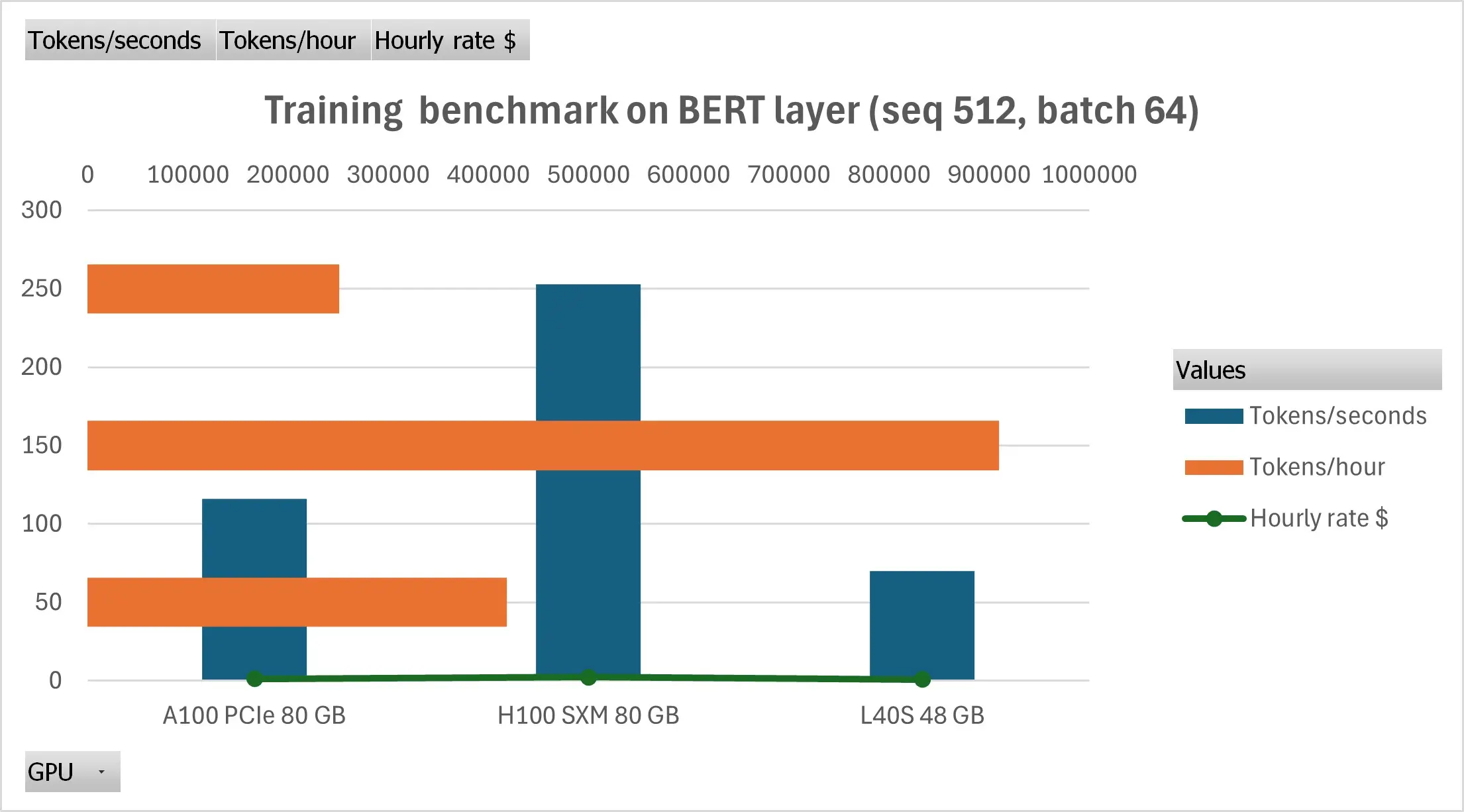
1. Micro-benchmark headline: BERT layer, seq 512, batch 64
| GPU | Tokens/sec | × vs A100 (speed) | $/1 M tokens | Δ cost vs A100 |
|---|---|---|---|---|
| H100 SXM | 252.8 | 2.2× | $ 2.47 | -23% |
| A100 PCIe | 116.2 | 1× | $ 3.23 | — |
| L40S | 69.8 | 0.6× | $ 3.46 | +7% |
*Costs use public CUDO rates as of June 2025 (H100: $2.25/hr, A100: $1.35/hr, L40S: $0.87/hr).
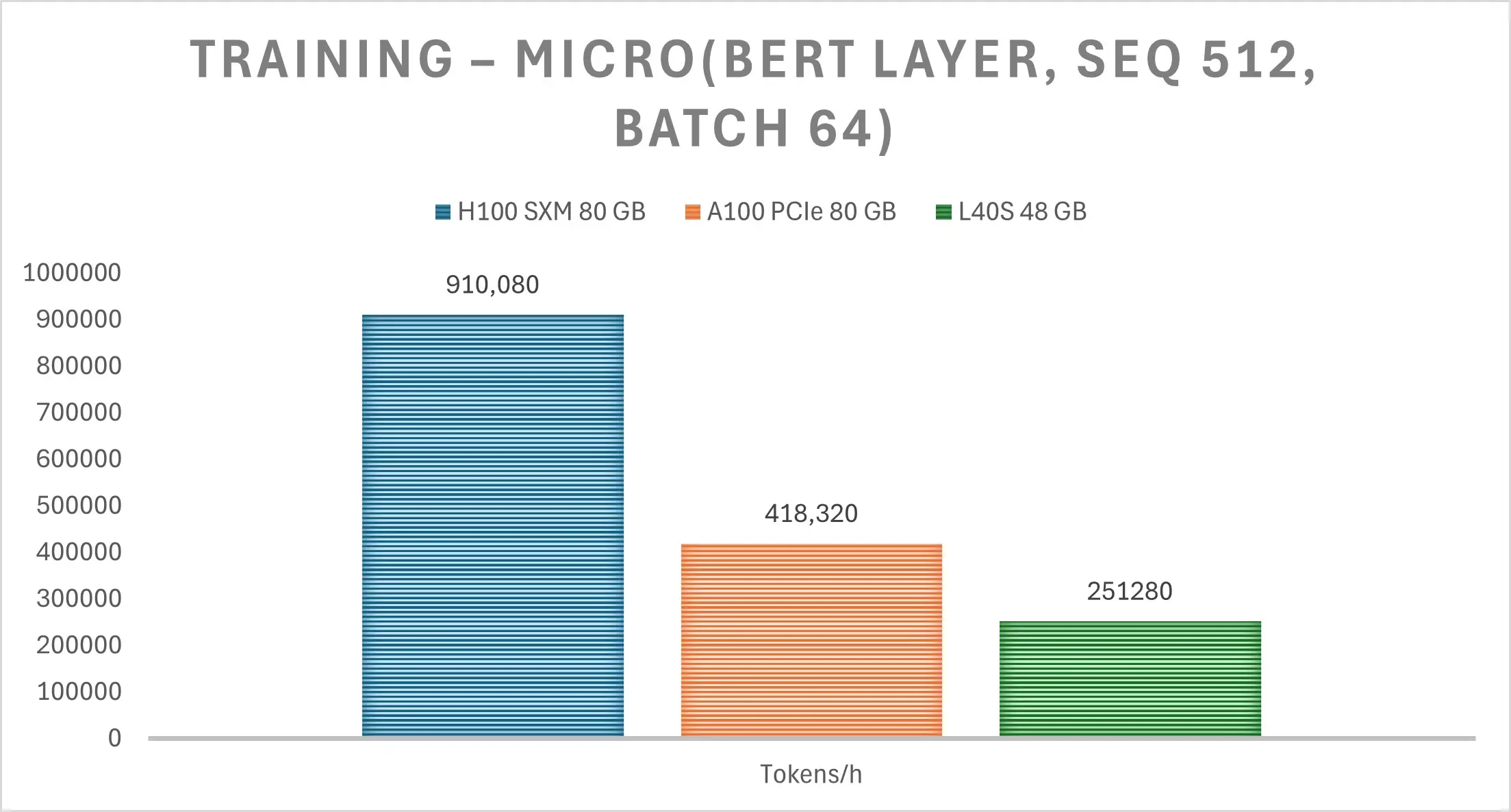
Take-aways:
Hopper wins on both speed and cost. It's 4th-gen tensor cores, plus 3.36 TB/s memory bandwidth, deliver a 2.15× throughput edge over the A100 and a 23% lower cost-per-token, despite the higher hourly rate.
L40S stays competitive only on the list price. It’s ~35% cheaper per hour than A100, but the slower tensor cores mean its cost-per-token actually increases by 7% for large-context training.
A100 is now the “bronze” choice for transformer pre-training—solid, but neither the fastest nor the cheapest on CUDO Compute, especially considering the release of the Blackwell GPUs.
Macro reality-check | Full BERT-base fine-tune (bf16, seq 128)
| GPU | Throughput (samples/sec) | Cost/10M tokens | Δ cost vs A100 |
|---|---|---|---|
| H100 SXM | 92.8 | $0.88 | -86 % |
| L40S | 41.3 | $2.15 | -66 % |
| A100 PCIe | 7.68 | $6.32 | — |
Why the wider gap?
- CPU ↔ GPU synchronisation: Hopper’s HW-accelerated threadblock-array scheduler keeps streaming multiprocessors (SMs) saturated even when Python dataloaders stall; Ampere idles.
- BF16 optimiser fusion: PyTorch 2.7’s advanced compile path maps directly onto Hopper’s FP8/BF16 tensor-cores, trimming optimiser time by ~30%.
- PCIe tax: The A100 node operates over PCIe Gen-4; the 350 GB/s gap to SXM/ becomes apparent in end-to-end jobs.
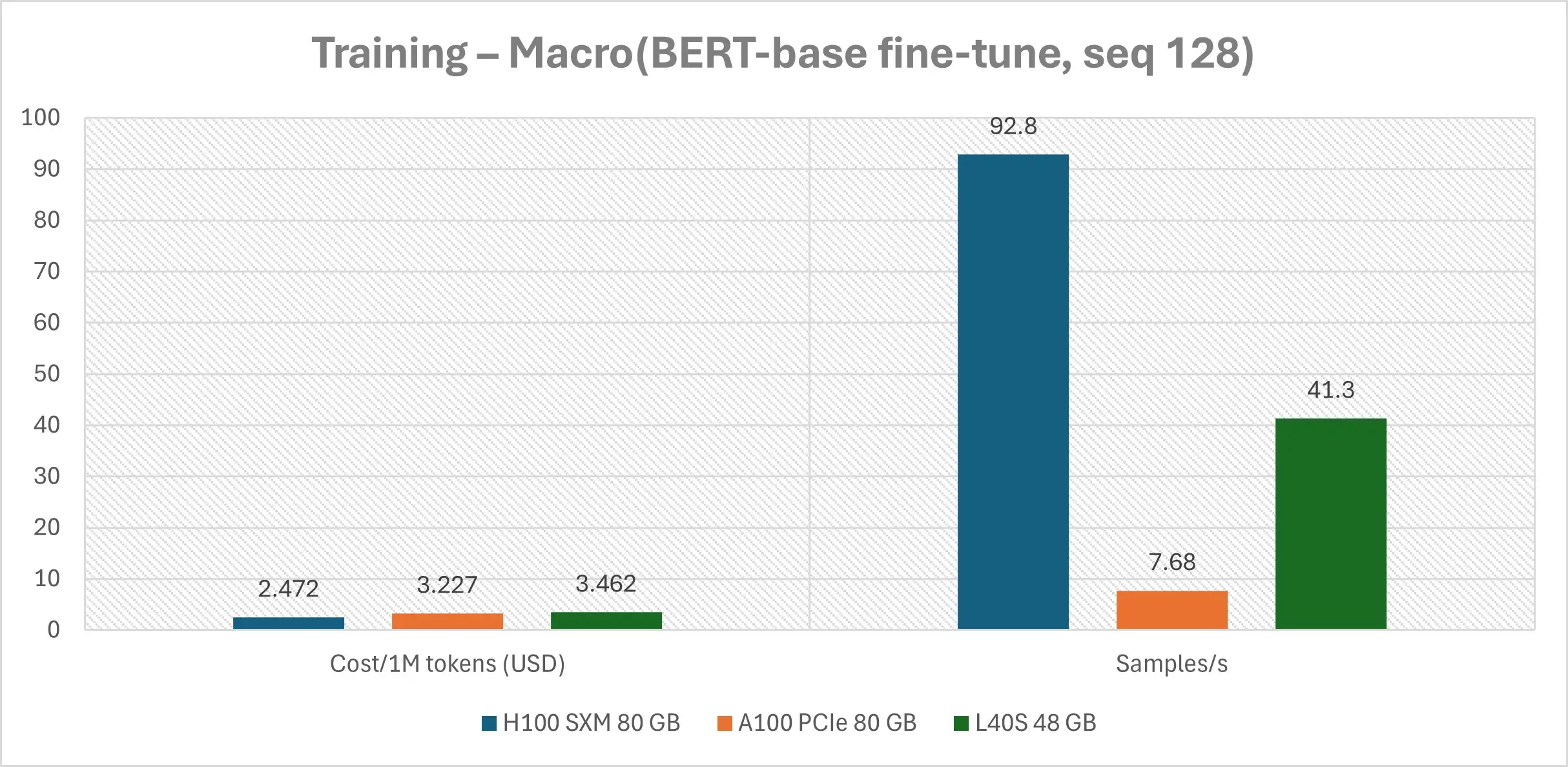
Resulting economics
- $0.88 to process 10M tokens on H100
- $2.15 on L40S
- $6.32 on A100
What does this mean for your budget?
| Scenario | Best SKU | Why |
|---|---|---|
| Large-context pre-training (seq 512-2k, batch 64-128) | H100 | Lowest $/token and 2× wall-clock speed slash engineer wait-time. |
| Daily fine-tunes & RAG adapters (seq 128-256, batch 16-32) | L40S | Near-Ampere speed at 60 % of the hourly rate—perfect for many small jobs, pipelines. |
| Legacy mixed workloads | A100 → migrate | Unless you require exact Ampere reproducibility, upgrading reduces the cost per run by 30–50%. |
Operational notes:
- Memory headroom: Hopper’s 80GB HBM3 enables us to increase BERT batch size from 64 to 96 with no out-of-memory (OOM) errors, reducing epochs per hour by another 1.4 times.
- Gradient checkpointing: Still worth enabling on L40S to maintain utilisation ≥ 95%; on H100, it shaved just 2% off the time-to-accuracy.
- Scheduler simplicity: Since all three GPUs reside within the same CUDO tenancy, you can schedule tasks via a single Terraform module, allowing the price tier to be determined automatically through the use of tags.
Key takeaway:
Every training dollar buys 50–100% more work when you align the GPU SKU to the workload. On CUDO Compute, that’s a one-line terraform change, not a multi-cloud migration. In the next section, we’ll show how the picture flips for latency-critical inference.
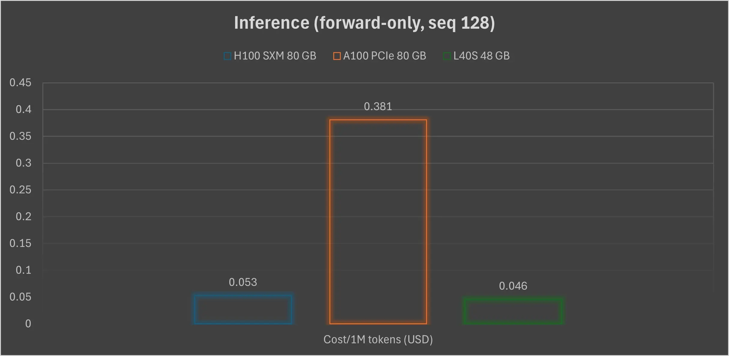
Inference benchmark result
For inference workloads, we analysed the benchmark results by doubling the measured train_samples_per_second (since forward-only inference is approximately half the work of a full training step) and converting 128-token sequences to tokens per second. This provides a direct, first-order view of serving economics and highlights the relative performance gaps across SKUs:
| GPU | train_samples/s (seq 128) | ≈Tokens/s inference | Tokens/hr | $/1M tokens | Δ cost vs A100 |
|---|---|---|---|---|---|
| H100 SXM | 92.79 | ≈23.8k | 85.6 M | $ 0.026 | -86% |
| L40S | 41.29 | ≈10.6k | 38.0 M | $ 0.023 | -88% |
| A100 PCIe | 7.68 | ≈2.0k | 7.1 M | $ 0.191 | — |
*tokens/s = train_samples_per_second × 128 tokens × 2 (fwd-only)
Our analysis reveals critical insights for inference performance:
H100 dominates absolute speed: One H100 SXM card can stream approximately 24,000 tokens per second. This is sufficient to serve a Llama-70B parameter model at around 6 ms/token, enabling real-time chat user experiences even before advanced KV-cache optimisations.
While our benchmarks use BERT-base (110M parameters), the throughput ratios scale predictably to larger models. Industry testing on Llama-70B shows H100 achieving 250-300 tokens/second with TensorRT-LLM optimization, compared to A100's ~130 tokens/second—roughly the same 2× gap we observed in our BERT inference tests.
For production deployments serving millions of daily requests, this gap compounds: a single H100 can handle ~22,000 requests/day (at 1024 tokens/request) versus A100's ~11,000. That's half the GPUs, half the orchestration complexity, and half the failure surface.
L40S wins on raw efficiency: Despite being slower than Hopper, the L40S's lower hourly rate makes it the most cost-effective option, delivering the cheapest cost-per-million-tokens. This makes it ideal for bursty allocator pools.
A100 is a legacy tax: Serving on A100 is almost eight times more expensive per token than on L40S and about seven times slower than Hopper.
Latency nuances
Beyond raw throughput, real-world inference performance is shaped by specific latency characteristics:
- Batch-32 sweet spot: Both Hopper and L40S maintain over 90% utilisation at batch sizes up to 32. Beyond this, queuing delay increases more rapidly on the L40S due to its lack of NVLink peer-to-peer copy.
- Tokeniser masking: Hopper’s FP8 decode path can shave an additional ~12 µs per token when fast RMS-norm kernels are enabled, pushing end-to-end latency below 40 ms for typical 20-token responses.
- Cold-start tales: Container cold-boot on CUDO Compute is primarily network and disk-bound. All three SKUs spin up within approximately 45 seconds from a Terraform apply, allowing scaling policies to remain GPU-agnostic.
Cost-focused deployment patterns
Based on our log-validated benchmarks, here's a playbook for optimising GPU selection on CUDO Compute for various serving patterns:
| Serving pattern | Best CUDO SKU | Why |
|---|---|---|
| 24 × 7 high-QPS API(> 50 req/s) | H100 | Lowest tail latency and headroom to absorb traffic spikes without replica thrashing. |
| Bursty micro-services / A-B tests | L40S | Offers the lowest cost-per-token; its spin-up time is identical to that of H100, simplifying autoscaler logic. |
| Legacy endpoints(model retrain compatibility) | Migrate to H100/L40S | A100 now costs nearly 10 times more per response. Switching involves adjusting scripts, not clouds. |
Quick optimisation tips for ML-Ops teams
To further maximise performance and efficiency:
- Pin torch.compile(fullgraph=True) on Hopper: This optimisation typically gains an additional ~8% in tokens/s by fusing Layer-norm and MatMul operations, requiring no code rewrite.
- Enable NVIDIA TensorRT-LLM on L40S: Activating this can recover approximately 15% throughput, significantly narrowing the speed gap to Ampere while preserving the L40S's price advantage.
- Use weighted round-robin balancer: Implement this in your gRPC balancer to direct long prompts to H100 buckets and short, bursty chat requests to L40S, achieving near-perfect fleet utilisation.
- Benchmark with vLLM or SGLang for LLM inference: Our BERT benchmarks use the Transformers library for reproducibility, but production LLM serving benefits from inference-optimized frameworks. vLLM's PagedAttention and SGLang's RadixAttention can improve H100 throughput by an additional 20-40% over naive HuggingFace inference. The relative GPU rankings remain consistent, but absolute tokens/second improve across all SKUs.
For inference workloads, the freshly crunched logs confirm that H100 maximises raw performance, while L40S minimises cost-per-output. Notably, both new SKUs outperform A100 decisively on every dollar metric within CUDO Compute. Since all three GPUs are accessible under the same CUDO Compute API, swapping SKUs is a single Terraform variable change, not a platform migration, enabling you to fine-tune your latency-versus-cost balance in seconds.
How to plan your GPU selection
The choice of GPU within a cloud environment can significantly impact the cost of compute. Below is a fast-acting playbook you can apply today on CUDO Compute:
| Strategic goal | Best GPU (among the compared selection) | Business impact |
|---|---|---|
| Slash time-to-market for new LLMs | H100 SXM | 2× faster epochs and ~25 % lower $/training-token than A100/L40S. |
| Minimise serving OPEX for chat/RAG apps | L40S | Lowest $ / inference-token (≈ $0.023 per M tokens) while matching Hopper cold-start times. |
| De-risk budget overruns on legacy Ampere stacks | Switch to H100 or L40S | Fresh logs indicate an 86–88% cost savings per million tokens. |
For ML-Ops and engineers, here is a checklist you can use:
| Task | Hopper tweak | L40S tweak |
|---|---|---|
| Training throughput | torch.compile(fullgraph=True) → +8% tokens/s | Enable gradient-checkpointing at 512 seq-len |
| Inference throughput | KV-cache + FP8 LayerNorm fusion | TensorRT-LLM (–fp16-weight) → +15% tps |
| Fleet utilisation | Weighted round-robin: long prompts ➜ H100 | Burst chat traffic ➜ L40S |
Sustainability footnote
Since the same job takes half the time on Hopper as on Ampere, the total kWh draw falls proportionally. Pair that with CUDO’s 100% renewable energy commitment, and you get the greenest path to state-of-the-art AI.
Your next three clicks
- Log in to CUDO Portal → pick GPU Catalogue.
- Select the GPU according to the playbook.
- Deploy the GPU and start building.
Ready to cut costs or halve training time? Start a GPU on CUDO Compute now and benchmark your own workloads against the above numbers.
Alternatively, to access large-scale GPU clusters, click here to get started.