Resources
Meta trained OPT-175B on 992 A100s over roughly two months. The longest stretch without an interruption in the run was 2.8 days. The team logged 35 manual restarts, more than 70 automated ones, and cycled over 100 hosts. All of this is documented in a 114-page logbook published alongside the model, which remains one of the most granular public accounts of what it actually involves to operate a frontier training cluster.
Buyers size a training run by theoretical GPU-hours and cost per token. Interruption overhead is straightforward to model on paper, but its two core inputs are not readable from the hardware.
The compute time lost per failure and the latency of restarting the job depend on how a cluster is orchestrated rather than on the underlying chip. Accelerators dictate theoretical peak compute, while the storage fabric, checkpointing frequency, and scheduler efficiency dictate the recovery penalty.
The only way to quantify them is to measure the cluster under load. The question that separates one operator from another is not whether the hardware fails, because the statistics of scale guarantee it will, but how much compute each failure costs.
GPU failure rate in large training clusters
Hardware failure at scale is consistent across all published runs, spanning models, vendors, and hardware generations.
Meta’s Llama 3 405B run used 16,384 H100s over 54 days and recorded 419 unexpected interruptions, roughly one every three hours, with 78% traced to confirmed hardware problems. GPU issues were the single largest category at 58.7%. Across the entire run, on more than sixteen thousand machines, there were two CPU failures.
Smaller clusters are not exempt; they simply fail less often in absolute terms. The BLOOM training run saw one to two GPU failures per week on 384 GPUs, though the team reported that spare nodes and three-hourly checkpoints kept the effect on throughput small.
At the other end of the spectrum, a 32,000-GPU deployment reported 678 unexpected interruptions, with HBM memory faults, PCIe device failures and NCCL watchdog timeouts alone accounting for 49.9% of all events.
The obvious reading is that reliability is deteriorating as clusters grow; the per-unit numbers say the opposite. Normalized to instance-hours, OPT-175B’s failure rate is roughly 0.0588% compared to Llama 3’s 0.0161%, an improvement of about 3.6x over three years. Absolute interruption counts rose because the clusters grew much larger, but the underlying silicon became more reliable per unit of time.
The failure rate is a statistical baseline rather than an operational anomaly, which means it is knowable in advance and can be planned around.
What breaks in a GPU cluster during training
Failures are often treated as a monolith, but they fall into three distinct classes, each demanding a fundamentally different response.
- Fail-stop failures halt the job: A GPU falls off the bus, an HBM error surfaces, a PCIe link drops, or an NCCL watchdog times out. These are the failures everyone plans for because they are loud and unambiguous. They are also the easiest to handle. The job stops, and the operator knows exactly when it stopped.
Root-causing them is harder than reading an error code because the signals overlap. Meta’s reliability study of its research clusters found PCIe errors co-occurring with XID 79, the code for a GPU falling off the bus, in 43% of cases on one cluster and 63% on another. The error code provides a symptom rather than a root cause.
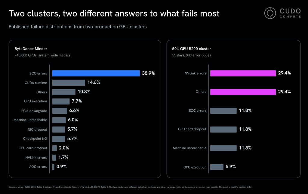
Failure distributions also differ between clusters. A 504-GPU operational analysis found NVLink errors to be the most prevalent single category at 29.4%, while a separate diagnostic study of large-scale training ranked ECC memory errors first at 38.9%. Both are credible, and the disagreement is the finding.
Failure profiles are a property of a specific cluster, its hardware generation, its interconnect topology, and its thermal environment, rather than a universal distribution that can be looked up. An operator who has not measured their own profile is planning against someone else’s. - Degraded nodes keep running slowly: A degraded node is worse than one that fails outright because, in a synchronous job, every other GPU waits on the slowest participant. A single node operating at 80% speed drags a sixteen-thousand-GPU fleet to 80% speed, and nothing in the logs registers a failure.
Meta’s reliability study identified what the authors call lemon nodes: machines that repeatedly cause job failures without ever failing outright. Detecting and removing them improved large-job completion rates by over 30%, an unusually large return for an operational practice that requires no new hardware. - Silent data corruption produces no error at all: This is the least understood class and the most expensive. The run continues, the loss curve keeps descending, and the corruption propagates directly into the weights.
Silent corruption accounted for 1.4% of unexpected interruptions during Llama 3 training. That sounds negligible until you account for the detection problem. The standard check is to watch for NaN (Not a Number) or infinity values appearing in the tensors.
However, a gate-level fault-injection study on a production-class data center GPU, running more than three million simulator hours, found that NaN and infinity outcomes account for only 1.01% of silent corruption events. The obvious check catches almost none of it.
In practice, the rest looks like a training run that behaves strangely without ever breaking. DeepSeek’s engineering team documented computational and memory errors not caught by ECC on their Fire-Flyer cluster, which surfaced as gradient-norm spikes, loss explosions, and, in some cases, a model that simply failed to converge.
In a 100,000-GPU deployment, 37 interruptions attributed to numerical issues were traced to seven hosts, with individual root-cause investigations taking several hours to multiple days.
The engineering time required for that debugging is also a real expense, not just the lost compute.
How often to checkpoint, and what recovery costs
Checkpointing creates a direct trade-off between saving too rarely, which lets every failure discard hours of completed work, and saving too often, which turns saving itself into a drag on the training time it is meant to protect.
The Young/Daly model is the standard reference for the optimum, and for a cluster of roughly 1,000 GPUs experiencing about two failures a day, it lands at one checkpoint every one to three hours.
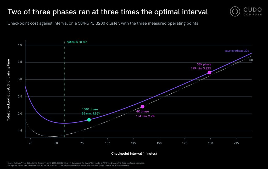
The measured numbers matter more than the model. An operational analysis of a 504-GPU pre-training run published the real figures:
- Checkpoint save overhead ran 18 to 31.7 seconds
- Mean lost work per abnormal termination was 0.98 hours, across 23 recorded cases
- Tightening the interval to 81.5 minutes brought total checkpoint cost to 1.82% of training time, against a theoretical optimum of 1.72%
Save overhead is small enough that shortening the interval is cheap, so the cost of checkpointing less often is usually borne in discarded work rather than saved in overhead.
Restarting is expensive rather than instantaneous because a checkpoint is not a single file but state sharded across every rank in the job. The optimizer state for an Adam-family optimizer is typically twice the size of the weights. A run with a few hundred gigabytes of parameters moves close to a terabyte of state on every save and load.
Resuming means reallocating the nodes, reinitializing the process group across all of them, reading that state back in parallel from shared storage, and then absorbing a cold first step while caches refill and the communication pattern re-establishes itself. Every rank has to complete before any rank proceeds, so the slowest reader sets the pace for the entire restart.
The cost of that sequence is not a function of cluster size. On a 100,000-GPU production system, it runs to roughly 10 minutes after optimization by teams who do nothing else. On a 504-GPU cluster, restart loading averaged 33 minutes, with a median of 31.
A cluster two hundred times smaller took three times longer to resume because of the storage path, the restart time, the checkpoint layout, and how much attention anyone has paid to them. This is why the techniques below aim to avoid a full restart rather than speed one up.
How to reduce the cost of each failure
The checkpoint interval is one lever among several. The other options fall into two groups: practices that are already well-known and widely used, and techniques that are still maturing.
Health checks and node draining
Pre-flight validation is the cheapest intervention available because excluding a node before a job starts costs nothing. Production practice combines several tools. DCGM diagnostics exercise the GPU, PCIe, and thermal paths.
GPU burn-in ensures sustained thermal stability. NCCL bandwidth tests confirm the interconnect performs at rated speed. Providers running this seriously go beyond a quick pass, executing 30-minute diagnostic loops and extended stress tests that run eight to twelve hours before hardware is released into available capacity.
Passing these checks does not guarantee a healthy node. A recent analysis of node validation methods found that burn-in tests exercise compute units with synthetic kernels over short durations without sufficiently stressing memory bandwidth, NVLink, or PCIe paths.
As a result, a node can pass the test while still exhibiting degraded intra-node communication under sustained load. NCCL tests have a subtler problem. The library’s own fault tolerance transparently reroutes traffic around degraded links, so a test can succeed while masking the very reduced bandwidth it was meant to detect.
One specific check is worth calling out because it directly relates to silent corruption. ECC must be enabled. A GPU with ECC disabled passes basic health checks but loses the mechanism that detects single-bit memory errors. PCIe link width and speed are worth validating for a similar reason, since a degrading physical connection auto-negotiates to a lower speed rather than failing, which is an early warning that appears as normal operation.
Lemon-node detection
A job that fails once tells you nothing about which of its several hundred machines was responsible, and a node that fails a health check has already declared itself. The nodes worth finding pass every test and are quietly present whenever a job goes down, so the only way to see them is to correlate failures with node membership across many sessions. That requires retained history rather than live monitoring.
On the 504-GPU cluster, three out of 63 nodes accounted for more than half of all exclusions across 224 multi-node training sessions. Meta found the same pattern at far larger scale, where identifying and removing repeat offenders improved large job completion rates by over 30%. A small number of machines cause a disproportionate share of the damage, so a small amount of analysis recovers most of the available benefit.
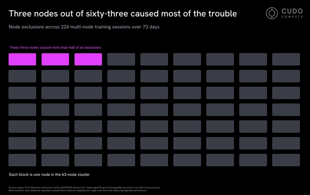
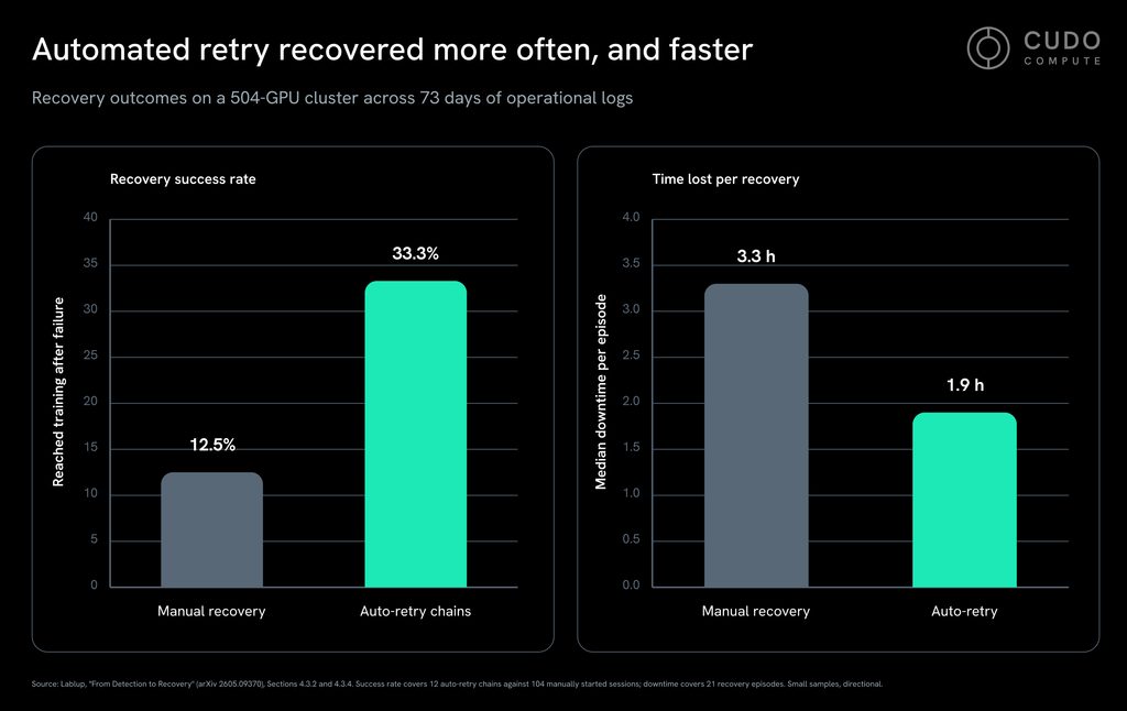
On that cluster, the exclusions were mostly deliberate, with operators manually isolating suspect nodes after noticing degradation across several sessions, because the cluster lacked per-iteration throughput instrumentation to automatically flag slow nodes.
The detection was human pattern-matching against memory. That is the honest state of most operations today, and it is also why the technique returns so much: it requires no new hardware, only retained failure data and the discipline to look at it.
Asynchronous checkpointing
Saving stalls training because the GPU cannot proceed while state is being written. Asynchronous checkpointing splits the operation into two steps: copying state from the GPU to host memory in a staging step, then writing to persistent storage in the background while training continues. Only the staging step blocks.
PyTorch’s distributed checkpointing documentation explicitly states that async saving increases CPU memory usage by the checkpoint size per rank, multiplied by the number of ranks, which can be a nontrivial amount of host memory for a large job. The technique is well established, not experimental. Systems built on it have demonstrated checkpointing every 14 to 19 iterations where synchronous saving would make that frequency unaffordable.
Just-in-time checkpointing
A more aggressive approach exploits a structural property of data parallelism. The same model state exists redundantly across data-parallel replicas. Rather than saving on a schedule, just-in-time checkpointing captures state at the moment a failure is detected using a surviving replica. Lost work drops to a single iteration rather than half a checkpoint interval.
Hot spares and elastic training
Two further techniques target restart cost rather than checkpointing. Hot spares keep provisioned nodes idle, allowing a failed node to be replaced without terminating the job. Elastic training continues at a reduced scale while a replacement is found rather than stopping outright.
Both avoid the full restart sequence, where the cost is concentrated at scale. Both are also less settled in production than the practices above. The spare capacity required by hot-swapping introduces a hardware cost that must be weighed directly against the restart time it saves.
Goodput: the number that governs training cost
GPU count and peak FLOPS describe a machine that never fails, and the rest of this piece has established that failures are certain. What governs cost is effective training time, the share of elapsed time a run spends actually making progress.
The useful property of goodput is that it decomposes. Google’s framework splits it into three layers, each answering a different question. Scheduling goodput measures how much time a job actually held the resources it needed. Runtime goodput asks how much of that allocated time was spent making progress. Program goodput asks how close the code came to the hardware’s roofline while it ran.
One definitional detail in that framework matters more than it first appears. Runtime goodput counts only progress saved in a checkpoint. Work completed between the last checkpoint and a failure does not count as productive because it does not survive. The checkpoint interval is therefore not a separate operational concern, distinct from goodput. It is one of the terms inside it.
Below the three layers is the more practical breakdown of where the lost time actually went. Google’s measurement library attributes badput to specific categories. These include accelerator initialization, training preparation, program startup, synchronous data loading, checkpoint saves, checkpoint restores, lost progress due to disruptions, and infrastructure recovery. An operator who knows which category dominates knows what to fix.
Meta held above 90% effective training time across the Llama 3 run. That figure came from straggler detection, fast checkpointing, and disciplined operations rather than the hardware, which failed every three hours.
Google’s infrastructure team estimates that for a typical training workload spanning thousands of accelerators for several weeks, a 1% improvement in goodput is worth more than a million dollars.
What execution cannot fix
Failure rates are a property of hardware at scale, and no amount of operational discipline eliminates them. A cluster of 16,000 GPUs will produce interruptions on a schedule regardless of who runs it, and the published rates are broadly consistent across operators, suggesting the floor is real.
What varies is not the failure rate but the cost. Between two clusters with identical hardware and comparable failure rates, the delivered training throughput can still differ substantially, because the cost of each failure is an operational variable rather than a fixed one. A failure that costs ten minutes and a failure that costs a wasted day are the same event handled differently.
The failure rate is fixed; the cost of each failure is not
Hardware sets how often the run will be interrupted. What the interruptions cost depends on the checkpoint interval, detection speed, the quality of the health checks, and whether anyone was watching the node that had been quietly slow for three days.
Each class of failure has its own answer: fail-stop failures come down to how fast the job restarts, degraded nodes to how fast anyone notices, and silent corruption to whether anyone is checking at all.
If you are planning a long training run, inheriting one that keeps stalling, or trying to figure out why your effective training time doesn’t match your GPU-hours, talk to our team about what it would take to close the gap.