Resources
There is no perfect machine-learning algorithm. They each lack something that others have, and we usually try to find the best one to solve complex problems. With ensemble learning, you don’t have to choose “the” model that best solves your problem because you can use all of them at the same time.
Ensemble learning is a technique that uses multiple models (of different kinds) to create one model. Think of it like this: a group of experts with different skills and perspectives can often crack a case that baffles any one of them alone. It is the “wisdom of the crowd” for machine learning.
In this article, we’ll break down everything you need to know about ensemble learning: its core concepts, the different types, why it’s so powerful, and how it’s being used in the real world.
If you’re facing a complex problem that no single model can solve, ensemble learning might be your answer. CUDO Compute is the platform for training and deploying your ensemble learning models with just a few clicks. Get started now.
The core concept of ensemble learning
With ensemble learning, you’re combining the predictions of multiple individual models (base learners) to create a single, more powerful model. Let’s explain this with a simple illustration.
You’ve got a mystery to solve, and you call in a bunch of detectives with different specialties. You get Sherlock Holmes with his sharp deduction skills, Miss Marple with her keen observation of human nature, and even Scooby-Doo and the gang (because who doesn’t love a talking dog?).
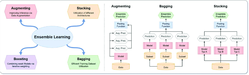
Illustration showing the four ensemble learning techniques: Augmenting, Stacking, Boosting and Bagging. Except for Boosting, all techniques are commonly utilized in modern deep convolutional neural network pipelines. Source: Paper
Each detective brings their unique perspective and methods to the table, and by working together, they can arrive at a more accurate and complete solution.
That’s what happens in ensemble learning. You gather a group of machine learning models – maybe a random forest, a neural network, and a logistic regression – each with its strengths and weaknesses to solve a problem.
Before we show how it works with some sample code, let’s discuss the different ways ensemble learning can work.
Ensemble learning methods
1. Bagging (Bootstrap aggregating)
Bagging is one of the most basic ensemble techniques. With bagging, you create a bunch of mini-datasets from your original data (with some repeats/crossovers) and train a separate model on each one. Then, you let them all vote or take the average of their predictions.
Basically, it averages the noise across models, making the overall prediction more stable and less sensitive to the specific training data. This is very much like having a bunch of friends give you their opinions on a movie. Individually, they might be a bit biased, but together, their average opinion is usually pretty accurate.
It also helps avoid tunnel vision (overfitting) by training on different parts of the data, making the model better and less likely to memorize the training set. Fair warning: while bagging helps prevent overfitting, it’s not a guaranteed solution for every overfitting scenario.
Here is an example of how it works using random forests, as it is the most popular bagging-based algorithm. It builds multiple decision trees, each trained on a subset of the data and features. The predictions from all the trees are either averaged (for regression tasks) or voted on and determined by majority rule (for classification tasks).
2. Boosting
In boosting, you start with a simple model and then keep adding new models that focus on fixing the errors of the previous ones. It’s like a video game character gaining experience and leveling up with each challenge.
It really produces very accurate models. When you’re using boosting, you start by training a weak model (e.g., a shallow decision tree). When the weak model makes a prediction, you identify the errors and factor that in (by assigning them higher weights).
You then train the next model, focusing on correcting errors. You’ll have to repeat this process until your model is very strong. Popular examples of boosting include:
AdaBoost (Adaptive boosting):
AdaBoost is like a teacher who pays extra attention to the students who are struggling. It works by training a series of weak learners one after the other (sequentially)—often shallow decision trees. Here’s the key:
- Focus on errors: AdaBoost assigns weights to each data point in the training set. Initially, all weights are equal. But after each model is trained, the weights of the errors (misclassified samples) are increased.
- Sequential learning: The next model in the sequence then focuses more on those “bad” examples, trying to correct the mistakes of its predecessor. This process continues, with each model adjusting the weights to emphasize the samples that previous models struggled with.
- Weighted voting: Finally, the predictions of all models are combined using a weighted vote, with models that performed better on the training data given higher weights.
This iterative process allows AdaBoost to create a strong learner by combining a series of weak learners that specialize in different aspects of the data.
- Gradient boosting
Gradient boosting is like a sculptor who gradually refines a sculpture by chipping away at the imperfections. It also works sequentially, but instead of adjusting weights, it focuses on minimizing the measure of error (loss function):
- Sequential error correction: The first model is trained on the original data. Then, the next model is trained on the differences between the true values and the first model’s predictions (the residuals). This means the second model is specifically trying to correct the errors of the first.
- Gradient descent: This process continues, with each new model focusing on the residuals of the previous model. Gradient descent is used to find the best parameters for each model that minimize the overall loss.
- Additive model: The final prediction is obtained by adding up the predictions of all the individual models.
By sequentially reducing the errors, gradient boosting creates a powerful ensemble that can capture complex patterns in the data.
- XGBoost (Extreme gradient boosting)
XGBoost is like the boss levels version of gradient boosting. It builds on the same ideas but adds multiple improvements to increase performance and scalability:
- Regularization: XGBoost has regularization terms to prevent overfitting, making the model more robust and generalizable.
- Tree pruning: It uses a more advanced tree pruning strategy to avoid creating overly complex trees.
- Hardware optimization: XGBoost is designed to use hardware resources better, making it faster and more scalable for large datasets.
- Parallel processing: It can use GPUs (parallel processing) to speed up the training process.
These enhancements make XGBoost a popular choice for ensemble learning, especially when dealing with large and complex datasets.
All three methods combine multiple weak learners to create a strong learner that outperforms any individual model. The specific strategies for achieving this differ, but the underlying goal is to improve overall predictive accuracy by using the individual models.
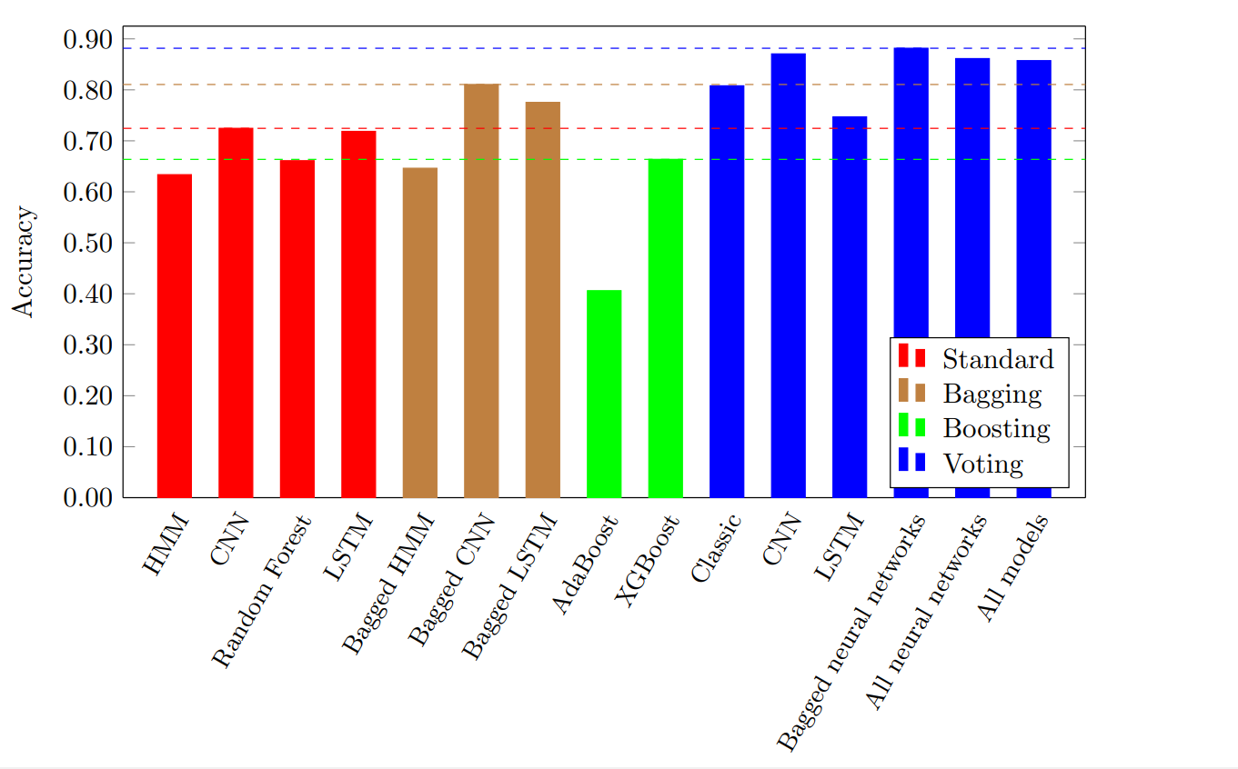
Shows that stacking techniques are beneficial, as compared to the corresponding “standard” techniques. Stacking not only yields the best results, but it dominates in all categories. Source: Paper
The computational demands of ensemble learning grow quickly. Boosting methods train models sequentially, which can bottleneck on single machines. Bagging and stacking, meanwhile, benefit from parallelization—training multiple base learners simultaneously across GPU clusters.
XGBoost’s support for multi-GPU setups makes it particularly suited for distributed training. When datasets exceed a single GPU’s capacity, distributing the workload across a cluster of GPUs reduces training time from hours to minutes. This is especially critical for hyperparameter tuning, where you might train hundreds of model variations to find the optimal configuration.
Infrastructure that supports elastic scaling—spinning up GPU nodes as needed and releasing them when training completes—makes ensemble methods practical for teams without dedicated ML hardware.
3. Stacking
Stacking is a very sophisticated ensemble method. You train a bunch of different models and then use another model (the “meta-learner”) to combine their predictions in the best possible way. The meta-learner learns how to combine the predictions of other models to achieve the most accurate result.
Suppose you have predictions from a decision tree, logistic regression, and an SVM. A meta-model (e.g., linear regression) can learn to assign weights to each model’s predictions to achieve the most accurate outcome.
It’s like having a smart manager who knows how to bring out the best in each team member.
4. Voting and averaging
Voting and averaging are simple ensemble techniques that combine predictions from all your models directly (we’ll see a bit of this later). There are main types of voting.
Hard voting is mainly used for classification tasks. The final prediction is determined majority vote among all models. Then there is soft voting, where you use the models’ predicted probabilities and average them to make a decision.
There are two times you really want to use this. The first is when you have multiple models that are already really good, so you implicitly trust them. The second is when you just want to be simple and have everything easily interpreted.
Those are the methods. Now, let’s see how it works.
How ensemble learning works
The first step is to decide what models can solve your particular problem and get them together. You can use any machine learning algorithm as your base learner, such as decision trees, neural networks, or support vector machines.
Side note: We will provide sample Python code as we go along, so we assume you have at least some knowledge of Python. Although these are not production-ready codes, they just explain the concept so anyone can follow along. We are also using scikit-learn models for ease of use.
The key is to select models that are diverse, with different strengths and weaknesses. For our code, we are using a neural network, a decision tree, and an SMV.
# Neural Network (MLPClassifier)
nn_model = MLPClassifier(hidden_layer_sizes=(50, 25), max_iter=1000, random_state=42)

# Decision Tree
dt_model = DecisionTreeClassifier(max_depth=10, random_state=42)

# Support Vector Machine (SVM)
svm_model = SVC(kernel="linear", probability=True, random_state=42)
The reason for selecting different models is that just like our puzzle-solving team needs different skills, your ensemble needs models with different strengths. Maybe one’s great at seeing the big picture like a decision tree (Mss Maples), while another’s good at finding hidden patterns like a neural network (Holmes). The variety helps you squeeze every last drop of information from your data.
If everyone on your team thought the same way, you’d probably miss some important clues. The same goes for ensemble learning. The more varied your models, the better they can solve your problems together.
Next, we trained each model separately on the same data (sometimes you can use different parts of the data for different models).
# Train individual models
# Train the Neural Network
nn_model.fit(X_train, y_train)

# Train the Decision Tree
dt_model.fit(X_train, y_train)

# Train the SVM
svm_model.fit(X_train, y_train)
Since the models themselves are different, how they interpret the data individually will be different, and as most machine learning algorithms have elements of randomness, even when they (the models) are trained on the same data, they’ll end up learning slightly different perspectives (parameters).
You could also say that each model needs to practice on their own before it can be combined. Using our detective illustration from earlier, it’s like having each detective investigate the case from their own angle.
After training each model, we test them to see how they perform. If you are satisfied with how they work, you can proceed to the next step: combining their results. There are a few ways the combination can be done (as we mentioned above). In our code, we used the voting method.
# Implement simple voting ensemble
# Collect predictions from all models
predictions = np.array([nn_pred, dt_pred, svm_pred])

# Perform majority voting
ensemble_pred = []
for i in range(predictions.shape[1]):
    # Take the column of predictions and find the most common value
    votes = predictions[:, i]
    majority_vote = np.bincount(votes).argmax()
    ensemble_pred.append(majority_vote)

ensemble_pred = np.array(ensemble_pred)
So each model votes, and we take the most common value (majority) as our prediction. The cool thing is, by combining these different perspectives, you often get a more accurate and reliable answer than any single detective (or model) could achieve alone. It’s like the Avengers assembling – they’re way stronger together than they are solo.
That’s how we used ensemble learning. If you want to check it out, here is the entire code:
# Import necessary libraries
import numpy as np
from sklearn.model_selection import train_test_split
from sklearn.datasets import make_classification
from sklearn.tree import DecisionTreeClassifier
from sklearn.svm import SVC
from sklearn.neural_network import MLPClassifier
from sklearn.metrics import accuracy_score

# Step 1: Create a synthetic dataset
# Generate a dataset with 1000 samples, 20 features, where 15 are informative and 5 are redundant

X, y = make_classification(
    n_samples=1000, n_features=20, n_informative=15, n_redundant=5, random_state=42
)

# Split the data into training (80%) and testing (20%) sets

X_train, X_test, y_train, y_test = train_test_split(X, y, test_size=0.2, random_state=42)

# Step 2: Initialize individual models
# Neural Network (MLPClassifier)

nn_model = MLPClassifier(hidden_layer_sizes=(50, 25), max_iter=1000, random_state=42)

# Decision Tree
dt_model = DecisionTreeClassifier(max_depth=10, random_state=42)

# Support Vector Machine (SVM)
svm_model = SVC(kernel="linear", probability=True, random_state=42)

# Step 3: Train individual models
# Train the Neural Network
nn_model.fit(X_train, y_train)

# Train the Decision Tree
dt_model.fit(X_train, y_train)

# Train the SVM
svm_model.fit(X_train, y_train)

# Step 4: Make predictions with individual models
# Neural Network predictions
nn_pred = nn_model.predict(X_test)

# Decision Tree predictions
dt_pred = dt_model.predict(X_test)

# SVM predictions
svm_pred = svm_model.predict(X_test)

# Step 5: Implement simple voting ensemble
# Collect predictions from all models
predictions = np.array([nn_pred, dt_pred, svm_pred])

# Perform majority voting
ensemble_pred = []
for i in range(predictions.shape[1]):
    # Take the column of predictions and find the most common value
    votes = predictions[:, i]
    majority_vote = np.bincount(votes).argmax()
    ensemble_pred.append(majority_vote)

ensemble_pred = np.array(ensemble_pred)

# Step 6: Evaluate the ensemble model
accuracy = accuracy_score(y_test, ensemble_pred)
print(f"Ensemble Model Accuracy: {accuracy:.2f}")
Now, let’s discuss the advantages of using ensemble learning.
Advantages of ensemble learning
Ensemble learning offers many advantages over using single machine learning models. :
1. Improved accuracy: This is the biggest (and most obvious) one. Since you’re combining the predictions of multiple models, you’re more likely to get higher accuracy than any individual model could on its own. Each model brings its own strengths and weaknesses, and their combined knowledge leads to better overall performance.
2. Increased robustness: Ensemble models tend to be more robust and less likely to overfit. If you want to know more about overfitting, we wrote about it here: overfitting article. As you train on different parts (subsets) of the data or focus on different aspects of the problem, ensemble methods reduce the risk of overfitting.
3. Better generalization: Ensemble learning models often lead to models that generalize better to new, unseen data because they capture a wider range of patterns and relationships in the data than a single model could. This improved generalization ability makes ensemble models more reliable and adaptable in real-world scenarios.
4. Versatility: Ensemble methods can be applied to different machine learning tasks, including classification, regression, and even unsupervised learning. They are also flexible in the types of base learners that can be used, allowing you to combine algorithms such as decision trees, neural networks, and support vector machines, as we did.
5. Reduced bias: Individual models can have inherent biases due to the specific algorithm used or the training data. Ensemble methods can help avoid these biases by combining models with different perspectives, leading to more balanced and fair predictions.
Combining the strengths of multiple models, ensemble methods overcome the limitations of individual algorithms and achieve superior performance in applications.
Challenges of ensemble learning
Despite its advantages, ensemble learning comes with certain trade-offs:
- Increased complexity: Combining multiple models requires more computation and memory.
- Higher computational cost: Training and managing several models can be time-consuming.
- Interpretability: Ensembles like random forest or gradient boosting produce “black-box” predictions, which can be hard to explain.
While ensemble methods are powerful, they should be used judiciously, considering these challenges.
Real-world applications of ensemble learning
nsemble learning, which combines multiple models to enhance predictive performance, have been adopted by various organizations across different industries. Here are some notable examples:
1. Financial Sector:
- Stock Price Prediction: Research has demonstrated the effectiveness of ensemble learning in forecasting stock prices for construction companies. By integrating models such as Artificial Neural Networks (ANN), Gaussian Process Regression (GPR), and Classification and Regression Trees (CART), predictions have become more accurate, helping investors make informed decisions.
2. Healthcare:
- Disease Prognosis: Ensemble learning has been applied to predict poor prognosis in patients with conditions like SARS-CoV-2. By combining multiple models, healthcare providers can better anticipate patient outcomes and allocate resources effectively.
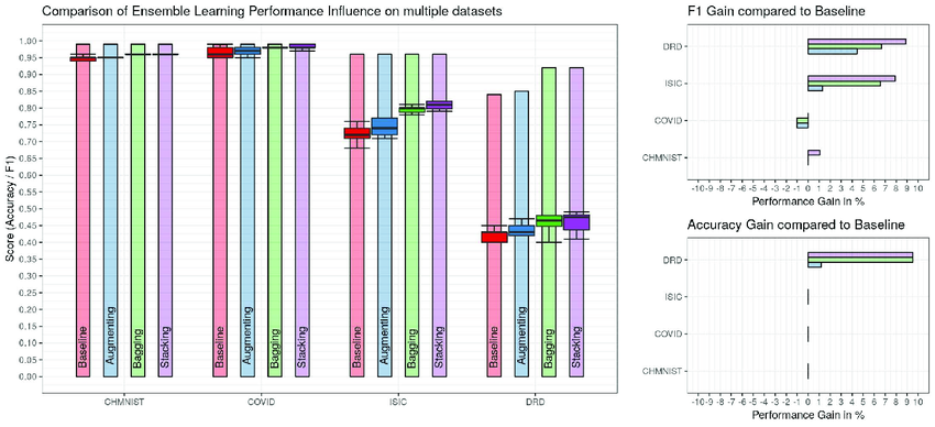
Comparison of ensemble learning performance influence on multiple datasets. Source: Paper
3. Environmental Monitoring:
- Ocean Wave Forecasting: Ensemble models have been used to improve the accuracy of ocean wave forecasts. By aggregating predictions from multiple models, researchers can provide more reliable information for maritime navigation and coastal management.
These are actual examples of how ensemble learning is being used to enhance decision-making and predictive accuracy across various fields.
Conclusion
Ensemble models are not just more accurate, they’re also more robust and better at generalizing to new data. And with it, you have a range of techniques to choose from. Bagging, boosting, stacking, voting – it’s like having a toolbox full of powerful tools, each designed for a specific purpose.
While it comes with issues like complexity and computational costs, its advantages make it worth it. And with CUDO Compute, the computational cost is not an issue. We offer the latest NVIDIA GPUs, such as the H200, and other cloud resources that make it easy and cost-effective to train and deploy even the most complex ensemble models, no matter how massive your datasets are.
CUDO Compute’s GPU clusters are built for exactly this. Scale from a single GPU to multi-node clusters as your ensemble complexity grows, with per-second billing so you only pay for actual training time. No reserved instances, no idle hardware. Start training your ensemble models now, or contact us for enterprise solutions.